"Loose lumber" diagnosis in Berlingo front shocks using accelerometers

By: Frank Rysanek [ Frantisek DOT Rysanek AT post DOT cz ] Measured and writtent during the spring of 2017.

Intro

I'm a proud owner of a Citroen Berlingo Multispace. Purchased new in early 2013, with a very low-end configuration of original options/accessories. Maybe substitute "love and hate" instead of the aforementioned pride ;-)

Among other interesting quirks, one lasting/recurring "issue" has been a kind of subtle knocking/rattling from the front suspensions on less than even tarmac. I don't mean outright jagged potholes, I'm speaking about smooth "waves", where the wheels still roll fine and normally you'd expect just a bit of silent "bobbing" and sideways tilt.
After four years of excuses from the authorized services ("that's okay, the front axle in the Berlingoes has always been noisy"), reading other people's semi-unfounded opinions and experience in the interwebs and watching the prices of aftermarket parts (esp. front shocks) slowly decline, to the tune of the problem getting gradually worse, in early 2017 I finally decided to speculatively replace the front shocks, which did indeed help. But that's just the "long story short".

Before I made that final move, being a computer nerd, I went a long way to properly narrow down the actual problem. I switched to an independent "garage" in the first place, where the techie owner was a little more talkative about the potential causes and common pains of these cars, compared to an authorized dealer/workshop. As all the car professionals have suggested, we started from the inexpensive measures:

• Obviously the first was a superficial inspection of the stabilizer and suspension parts.
• Some people (car owners) in the internet fora shared an experience, where a problem of this kind was caused by the upper "safety dish" on the strut's piston rod:
  
  = the very last washer, with a rubber collar, on the front strut upper mount, whose sole purpose normally is to prevent the strut assembly from dropping out of its "dome" if the car gets lifted for tyre replacement (or in case of an incidental jump). Some people have claimed that this needs to be tightened more, other people suggested au contraire that it needs to be "spaced higher up" using an additional washer underneath, because due to the stupid construction, this original rubber-lined washer tends to rap against the "dome" from above, and after some time, the rubber lining gets chewed off and the washer starts ringing hard against the dome... and an original replacement, even an "upgraded" version with more rubber, doesn't quite solve the basic problem...
  By comparison to other car models, such as some Skoda and VW that are "the expensive domestic brand" where I live :-) I noticed that the washer could indeed use "more rubber". And I managed to improvise a workable alternative safety dish along those lines:
  
  This replacement actully consists of two items: the metal part is a VW/Skoda part no. 1J0412319c , combined with a particular wastewater sealing from a plumbing shop, known locally as "E-1432 by Nyvlt" (probably not exported outside our domestic market).
  The hole in the VW dish is just right for the 14mm piston rod (probably a standard diameter) and I've actually tried three different rubber seals, tested them on the road, before settling on the particular model mentioned above :-)
  
  From those experiments, I also have a video of how the front strut upper mount moves during normal operation = during a ride. It shows how it tilts between extreme left and right positions of the steering mechanism, as well as some residual motions (allowed by the upper mount) of the piston rod during a ride on a rough road. (Note: the washer assembly in this video is not meant as a final solution! This was only chosen for demo purposes, for a good visibility of the relative motion / vibration, and the demo ride was not on public roads.)
  Overall the contemporary upper mount assembly seems to be a cheap construction. In the good old days, the upper mount "constructional dish" (seat of the axial bearing) used to be bolted at two or three points to the chassis dome. Not sure if there's any direct consequence with vibration transfer from the strut assy to the chassis.
  The morale from this exercise was, that the choice of the rubber spring/seal/bushing on that topmost safety dish does have some limited influence on the vibration transfer to the chassis, but is definitely not the main source of the problem. If I tried riding the car without the safety dishes, in my case the rattling noise was actually louder. But a hard rubber bushing ring also resulted in loud rattling. Moderately hard rubber resulted in least noise.
• Next, we speculatively replaced the sideways stabilizer links ("bones" as they're called around here) - the replacement was an "HD" variety by Meyle, just to be on the safe side.
  This did not affect the rattling behavior in any way.
  This is not surprising - the originals were still pretty stiff at the ball joints.
• I got myself some analog accelerometers, and before and after the final shock replacement, I have managed to record vibrations at both ends of the left shock. Which allowed me to do some analysis afterwards. This is in fact the central topic of this paper. Read on if interested.
• We have not tried replacing the stabilizer rod bushings - these looked allright. The techie replacing the shocks also opined that the upper mount (bearing and its "seat dishes") were in perfect order and did not need replacement. He actually said the same about the original shocks, but he likely meant "okay" in terms of damping and remaining oil-tight. My vibration recordings seem to point quite clearly to the shocks as the source of the knocking. More on that below.

The shocks

At the front, just like many other cheap cars, the Berlingo has McPherson-style struts, with twin-tube oil and gas shock absorbers as the "damping" element.

Setup of the sensors

During the months when I was scratching my head over the front suspension, I was fortunate to come across some cheap accelerometer sensors: the MMA7341LC, conveniently mounted on tiny PCB's by Pololu (model 1247).

The voltage coming out of those analog sensors is suitable for AC-coupled input into a PC soundcard "line in", and the acceleration range (9G) also happens to be just enough for my application. The bandwidth of "DC to approx. 1 kHz" was plenty good enough as well.
I was interested to sense vibrations at two places: at the shock's top end and bottom end. Therefore, I used thick double-sided adhesive tape (with a foam "substrate") to stick the pololu boards to a "carrier bracket" made of soft aluminum sheet, and I strapped those brackets to the shock tube (at the bottom) and to the piston rod nut (at the top) using plastic zip ties.

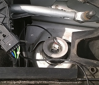
I needed to sense vertical vibrations at two places, and I only had a stereo input anyway (in an older notebook PC, which still had three stereo jacks at the front) - so I had to pick one of the three outputs at each accelerometer: obviously the output for the axis that happend to end up being "vertical", as a result of the sensor's mounting position (X and Z respectively). And, with only two channels, I could only record one shock at a time. I chose the left side.
I breadboarded a simple interface, to provide filtered power to the two sensors (using a 78L33 stabilizer from USB power), AC coupling of the sensors to the soundcard, and to serve as a wiring converter.

First data

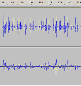
At this point, let me present two clear examples of the raw audio recording:

• The factory-original shock before replacement (Sachs - at 30 000 km / 4 years of age)
• A new aftermarket shock after replacement (KYB/Kayaba)

Raw accel data zoomed out	The original	The new one by Kayaba
Upper track (left audio channel): acceleration at the top of the piston rod. --- Lower track (right audio channel): acceleration at the bottom of the shock = shock outer tube, linked to the wheel hub

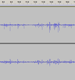Click the thumbnails to get a full screenshot of Audacity.
If you want to zoom in on the details in time, you will need Audacity or some other audio viewer/editor.
Some screenshots at a closer zoom:

Raw accel data zoomed in	The original	The new one by Kayaba
Upper track (left audio channel): acceleration at the top of the piston rod. --- Lower track (right audio channel): acceleration at the bottom of the shock = shock outer tube, linked to the wheel hub

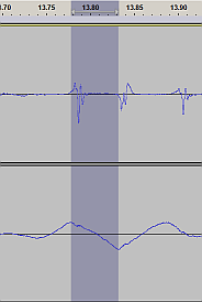The data is fairly raw, only cropped (the most interesting section in time of the original total footage) and inverted (the fist post-processing step, more on that below.) These two examples correspond to a part of my "test track" where the "loose lumber" noise is the most audible, and the character of the imperfection on the road surface (smooth waves) is just right for problem reproduction.

I took special care to use the same input gain in the recording software, so the amplitude scale is identical between the two recordings (except for the fact that I probably rode about 15% slower with the new shock).

I recommend that you listen to the recordings using some plausible earphones. It's true that no earphones will allow you to hear the cca 15 Hz at the wheel (the tarmac waves) but even those subsonics aside, the signal is still pretty heavy with low frequencies. My Koss Porta Pro apparently does a good job. The built-in speakers in a notebook PC do not work very well for this signal.

The signal does not contain a pretty "stereo landscape" - instead, the rattling is prominent in the left channel, and the right channel is practically all just subsonic "pumping" (of which you can hear the very top end, percieved as an unpleasant and constant dim thunder). When viewing a stereo track in Audacity, the left channel is at the top, and the right channel is at the bottom.

Post-processing and further analysis

I was using Audacity throughout the process: first to capture the raw audio, and then during several stages of "signal refinement": DC offset and slope removal, amplification, spectral analysis...

Before actual measurements, I determined by a simple test that I needed to invert the signal, so that upward acceleration now results in a positive value of the signal.

Note that the output of an accelerometer is, that's right, acceleration. The acceleration signal already happens to correspond quite neatly to my human auditory experience in the car, but having a semester or two of college-level maths (combined with high-school physics), I was curious if I could integrate the acceleration data back into velocity and indeed absolute position.

Audacity doesn't seem to contain a filter for "ideal integration" - though the operation has some strong low-pass properties :-)
So I wrote my own integrator - I wrote a simple C program in mingw32-gcc that takes a .WAV file as input and produces an integrated .WAV output. The only other parameter is an output "divider". The .WAV file format is 16bit and my integration program uses a 32bit internal "accumulator" as a workspace for its simple "discrete-time signed integer sum" operation. The program does not automatically divide the accumulated result by the sampling frequency or anything like that - the user has to specify a divider at the command line. The program does not do DC offset removal or any other such "normalization", except for the final "divider" to make the output from the 32b accumulator fit into a 16bit WAV file. Therefore, DC offset removal is up to the user - I did this in audacity, either using the "normalize" filter, which has an option to remove DC, or using a high-pass filter with a roll-off of maybe 0.5 to 2 Hz.

Playing with the discrete integration was fun. This is something we never did at school (you know - economics and IT). It was fun to see the integration work on arbitrary data, and see the theoretical integration formulas in action. Examples of what I could observe (and sometimes had to correct):

• a DC offset in the input data - results in a positive slope across the output time series
• a slope in the input data, centered around 0 (DC offset removed) - results in a "bow" across the output file
• any DC offset or a slope across the input dataset or even a very low frequency "fluctuation" would result in large swings getting accumulated in the output, which would easily outgrow the interesting phenomena that I was after in the first place. Thus, removal of any DC or near-DC components in the input time series is pretty much a necessity :-(
• sine-like wavelets in the input data would get phase-shifted by 90 degrees in the first-order integration, and would get effectively inverted after the second-order integration. Textbook stuff, really.
• a sharp spike in the acceleration data would result in a sharp angle in the integrated velocity data, which in turn would transform into an abrupt "step" in the 2nd-order integrated position data.

At first I considered using equal dividers (= scaling constants) and filtering operations on both my "data sets", but after some time of trying I gave up and just tried to keep the resulting amplitudes "normalized" to an almost maximum value, to make them nicely visible in Audacity.
I even split the stereo recordings into mono tracks and processed each channel separately, for better visibility of the phenomena I was looking for. Thus, the final detailed six-track screenshots don't keep any sort of scale. No fixed scale between "top and bottom" (speaking of sensing positions on the shock absorber) or between "before and after" (shock replacement) or between the three "stages of data integration".
I also zoomed in on just a few seconds where the phenomena were particularly well demonstrated - which locally allowed for yet more normalization and amplification, compared to what would be possible across the whole dataset. At the same time, it is debatable if localized DC removal (after integration, to allow for greater AC amplification) removes some of the information, previously achieved by integrating over a longer interval in time - shifts zero crossings for one thing. At a conceptual level, the DC offset is a part of the "constant" on the output of integration and is therefore arbitrary anyway = we are "free to choose the zero reference point" :-)
For visibility end explanation of the short transient events, this "maximum detail" approach is better than "staying faithful to the uniform scale". After all, the basic loudness "before and "after" is easily visible (and audible) in the raw data. You can also let Mr. Fourier show his muscle, if you don't believe your own ears. I did use the spectral domain to confirm my estimates, what frequencies I can see in the time-domain data (tarmac waves and the rattling glitches/wavelets).

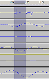
Time to look at some data.

Integrated data, top/bot to scale	The original	The new one by Kayaba
Acceleration - piston rod --- Acceleration - shock tube --- Velocity - piston rod --- Velocity - shock tube --- Position - piston rod --- Position - shock tube

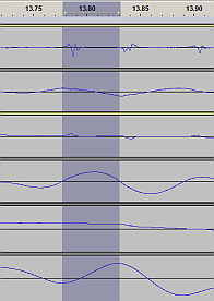In the "display arrangement" above, I kept the vertical display height equal for all the tracks, and I kept the "piston rod vs. shock tube" = top vs. bottom scale faithful to the original, within a stereo track, within an integration step.
I did not keep scale across each of the two integration steps: I removed DC before each integration and I normalized the resulting stereo (both channels in stereo amplified by the same constant) to use the available bit depth / signal range.
I actually did some limited high-pass filtering, to get rid of some very low frequency waves (spanning many seconds) which would otherwise hog all of the vertical resolution and obscure the fast and relatively low-amplitude transient events (ripples, wavelets) that we're interested to see.

That's really the main problem. If you want to "see what the motion really looks like", to see the whole picture, inevitably your view will be occupied by the lowest-frequency waves, as these have the highest amplitude.
The fast ripples that cause the rattling are relatively smaller in amplitude. The apparent paradox, that the "tiny" ripples are so well audible to our ears, has to do with the frequency range of our ears and also with the "physiological sensitivity curves" (known by the names of their authors Fletcher and Munson, though they were not alone in that research).
Also consider that the slow bobbing of the chassis does not translate into (that much) infrasonic accoustic pressure inside the cab, as the chassis "dances" as a whole, the structure of the cab is stiff at that wavelength, so the bobbing does not result in volume changes of the interior compartment. And the bobbing motion is so slow that we sense it with our butt, rather than our ear :-) (Actually - the vestibular sensor in the inner ear, effectively an accelerometer and tilt sensor, does play a role, just as well as some force/tension feedback sensors in our skeletal muscles).
On the contrary, the rattling/rapping/knocking vibrations have a short enough wavelength to excite individual car body parts into accoustic radiation, which enters the cab interior - and the frequencies are in the audible spectrum. They enjoy more gain at the transmitter and at the receiver :-)

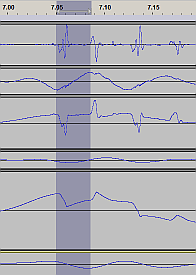
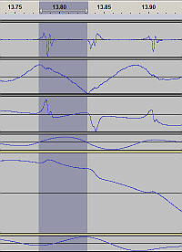
In the following screenshot, the tracks are individually normalized for maximum amplitude (I've split the stereo), and their "display heights" are also modified, for a better visibility of... important stuff :-)
Namely, the bottom-end (shock tube) tracks are fairly boring, pretty close to a perfect sinewave, so a fairly small display height is enough to get the basic idea - but the top end (piston rod) recordings are where the interesting rattle takes place, and of them, the "position" version (after double integration) is perhaps the most intuitive to understand - or, the most interesting to analyze :-)
Even in this picture, the integrated tracks have gone through some high-pass filtering (on top of DC removal) to make rattling stand out more from the "base signal" (slow and deep tarmac waves).

Integrated data, each track individually normalized	The original	The new one by Kayaba
Acceleration - piston rod --- Acceleration - shock tube --- Velocity - piston rod --- Velocity - shock tube --- Position - piston rod --- Position - shock tube

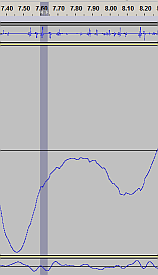
In the following screenshot, I have further focused on the "top end = piston rod position", which now takes most of the screen real estate. For this picture, I have re-processed the data without high-pass filtering - just the double integration interleaved with DC removal. Thus, you can see the subsonic bobbing with the faster transients all in one picture.
For "timebase reference", I have kept the piston rod acceleration track, and the shock tube position, also in the picture (minimized).

Integrated data, selected tracks, focusing on the piston rod position	The original	The new one by Kayaba
Acceleration - piston rod --- Position - piston rod --- Position - shock tube

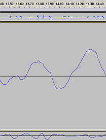Compare the waveform of the "position - piston rod" to the previous screenshot, where the subsonic wave had been filtered away.
Can you see where the piston rod suddenly "jumps down" and then moves on along some slower "sine wave", only to suddenly "jump back up" a moment later, and then follow that slow smooth sine wave again? Unsurprisingly, those sudden jumps in position correspond to the "rattles" = to the sparse and fast glitches in the acceleration data. Unsurprisingly, because effectively the acceleration and position are just two different forms of the same data (the transform between them being a double integration / derivative).
Note how the acceleration glitches (rattles) at the top sensor are correlated in time to the "position" waveform of the bottom sensor (shock tube, coupled straight to the wheel hub). The rattles appear to occur at the top and bottom peaks of the "road wave" amplitude, or just slightly after the peak.
Also note, how the three forms of the bottom sensor signal (acceleration, velocity, position) neatly document the schoolbook formula for integrating a sine wave: sin(x) -> -cos(x) -> -sin(x) :-) For the "glitches" (wavelets), the visual result of the integration is perhaps not so pretty and immediately obvious, as the wavelet is a relatively complex waveform.

In the last picture, you probably know what you're looking at: the audible "position jumps", superimposed on some subsonic sine wave. I believe that in this particular picture, the slow wave corresponds to the car body "bobbing" on its suspension, while riding over uneven road. The combined waveform depicts the car body hovering on its suspension (that's the large slow wave), summed with the tiny movements of the shock's piston rod in the strut's upper mount (= relative to the chassis).

In the various waveforms depicted above, there are several noteworthy frequency components:

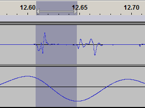
At the bottom sensor (shock tube), the most prominent spectral component is obviously the unevenness of the road. We have previously established, by practical tests (and seconded by one previous publication) that the rattling noise of interest is best reproducible on relatively even tarmac, no outright potholes, just getting a little wavey from heavy trucks or some such. No sharp edges on the tarmac, just smooth waves. And, the ride speed should be such that the frequency of the tarmac waves is broadly around 15 Hz = period of about 70 ms.
At the top sensor, in the "position" track you can see the sudden jumps, correlated to the 15 Hz "basic road wave" (as mentioned above), but the most prominent spectral component is actually a slow wave, roughly 2 Hz or so, which looks like the inherent frequency of the car chassis hovering and tilting on its suspension.
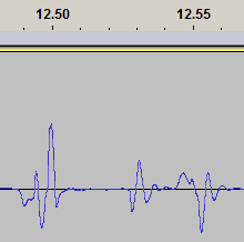
The audible glitches actually seem to be short wavelets, with a frequency of about 200 Hz. Short pulses of this - that's the rapping noise, in temporal and spectral domain. This is what the cochlea in the human ear responds to, and what the brain then interprets as "something going knock knock knock or rattle rattle".

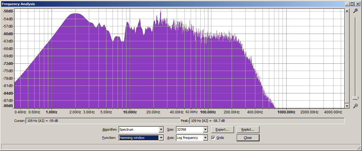
And yes you can have Audacity calculate the spectrum for you... but you'll find out that the precise spectrum depends heavily on your selection of the time series subsection to transform, on window length, on the windowing algorithm etc. Welcome to the subtleties of FFT.

Spectra	The original	The new one by Kayaba
Acceleration - piston rod
Acceleration - shock tube

(Please note that the vertical scale is different per picture. You need to zoom in = click the thumbnail.)

Are we there yet ? Any conclusions ?

Unfortunately, the data available, and the "analysis" outlined above, do not amount to enough clues to draw some overwhelmingly definitive conclusions.

Looking at the "position" traces of the upper sensor (piston rod), without additional clues, I can come up with two explanations for the observed jumps:

1. The upper mount theory.
   The jumps could be a sign of some "bounded flexibility" in the upper mount. Combined with static vs. dynamic friction of the piston inside the shock housing.
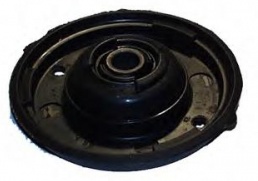   Consider that, when assembling the strut, the upper mount's "rubber dish" (really a steel dish coated in rubber) holds the spring somewhat compressed. The assembly is held together by the "last but one" (lower) nut on the piston rod. Released from the "spring retractor aid", the spring extends as far as the shock allows (with piston rod at maximum extension). The "residual" spring compression force can be a couple hundred kg, enough to kill a careless techie upon improper disassembly of the strut... I mean to say that the flexible joint in the strut's upper mount dish is probably quite tough...
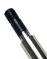
   Only when loaded by a car body, does the piston rod slide somewhat inside the shock, and the upper mount's dish center gets relieved of the permanent static axial load from the spring. And such are the conditions of normal operation. The upper end of the piston rod is tightened by a nut (against a seat of sorts, at the lower end of the piston rod thread) into a metal bushing that's fused into the rubber of the upper mount's main dish. The rubber mass around this bushing ring does allow for some tilt, and likely also some axial freedom. Without some closer inspection, it's not clear if this bushing (or is it a bearing?) can start rattling in the dish or something.
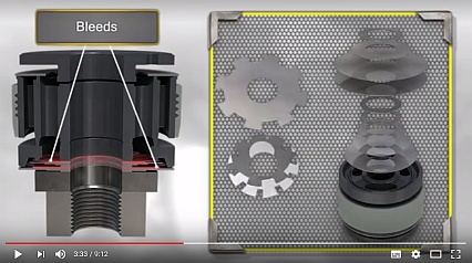
2. The shock absorber theory. (The excellent training video on YouTube, linked below, was created by Monroe.)
   = my other possible theory is, that the jumps and the audible "clicks" are a sign of something going on inside the shock absorber.
   Namely, a standard twin-tube shock absorber contains several valves on the piston and at the base, that open and close (or throttle) depending on "flow rate" = piston motion velocity. This is to achieve a non-trivial curve of hydraulic resistance, or force vs. flow rate. Hydraulic resistance of a hole or a section of pipe ordinarily grows with flow rate (velocity) - this is in contrast to electric resistance, which is constant (independent of current). Thus, oil pressure (or piston force) as a function of flow rate, on a simple hydraulic resistance, would ordinarily be quadratic. The degressive valves are there in the shock to make the hydraulic resistance more constant, or even slightly decreasing at a higher flow rate.
   The degree of throttling (hydraulic resistance) in the shock valves is also made dependent on flow direction. This is to allow for a relatively easy-going compression, taking turns with a relatively tight throttle on rebound = to allow for a soft absorption of a bump, but also to prevent the vehicle from jumping on "rebound" (or, to improve the average oscillation damping factor across the whole cycle of compression+rebound).
   One possible explanation (rather naive) might relate the "jumping" of the piston rod to the asymmetry between compression and rebound forces: as the wheel hub stops compressing the shock and begins rebounding, the initially steep throttling rate tugs heavily at the upper mount, only to relieve a bit, once the speed grows higher - and the reverse process hapens as the rebound phase slows down to a halt and turns into another compression.
   But reality is probably more complex than just that. Perhaps it's time for a bit of shock curve-tracing basics :-)

Shock absorber characteristics - "Dyno" measurements and charts

The charts in this chapter are all "for illustration only". They are by no means based on some measurements of my actual shocks. There are companies in town that offer dynamometer measurements on commercial basis, and it would probably be the one right way to go, but I don't feel like spending further money on this :-) The waste of time is enough.
That said, let's get back to the topic.

As usual in systems with some impedance and dynamic energy, especially in resonant systems (such as the mass of a car body on suspension springs) it's always somewhat difficult to say what was first: force, or motion? In our case, is force a function of motion, or is it the other way around?
Theoretically it's a bit of both at the same time :-)

Technically in a car suspension system, the "mass vs. spring" resonant system (and its characteristic frequency), and the "car body vs. road profile" relative motions and inertia, will probably be dominant, setting the coarse velocity patterns of the shock.
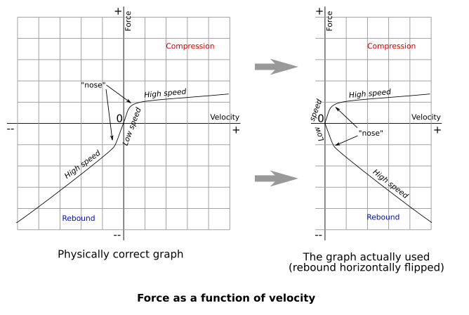
As a result of the relative velocity applied, the shock absorber responds with force. Hence the first chart - possibly the key chart to characterize a shock absorber.

To me as an outsider, the four-quadrant form of the chart seems more obvious - yet the dynamometer tools (or dynoes) seem to follow their own tradition of producing a two-quadrant chart, where the rebound section is inverted. Once you're aware of that, the traditional dyno graph of "force as a function of velocity" feels perfectly allright :-)

Notice how the shock supposedly starts moving with a tighter throttling factor (relative to velocity), only to open more when reaching a particular "infexion point". Such an inflection point can exist in either half of the chart (or, may not exist at all?) and it's called the "nose".
There's an excellent introductory paper on the topic, containing deeper analysis and examples of these charts. I've just re-sketched the two pictures around here to have some material of my own.

The dynamometer typically consists of some linear guide structure for the shock that gets set in motion by a conventional constant-RPM electric motor, driving an excentric drive or cam that translates the steady rotational motion of the "cam" to the linear compression/rebound motion of the piston rod (of the shock under test). The motor is a source of a sinusoidal motion (position and speed) that gets applied to the shock.

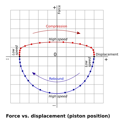
The raw low-level signals available from a dyno appear to be position (aka displacement) and force, rather than velocity vs. force. Hence the second chart.

This chart does not have time on either axis, neither pure time, nor implicit in velocity. But, mind the "points" on the force/displacement curve: they are sampling points: isochronous points in time where the measurements are taken. Therefore, the horizontal (displacement dimension) spacing between the sampling points means velocity. Note that if the motion is uniform and circular (sine and cosine combined), the velocity is "90 degrees shifted" after the displacement "signal" (which is the lateral axis in this chart).
Consider that you want to morph this into a force/velocity chart. You could combine the known RPM and eccentricity radius to obtain the displacement signal, and derive the velocity from Δ displacement sampled at isochronous sampling points. From a different point of view, given that the drive motor's RPM is constant, it is also possible to phase-shift (delay) the displacement signal by a quarter revolution, which should also result in a velocity signal.
The force could theoretically be measured by a tensometer sensor, but practically it's likely derived from electric consumption (current) at the motor. It's a dynamometer, see?

Yet the chart of "force vs. displacement" may actually be easier to obtain (with less computing) and can show many problems just fine.
Consider a shock absorber with an ideally constant hydraulic resistance, i.e. the force is precisely proportional to velocity (multiplied by some constant). In the force/velocity chart, this is a straight line passing through the zero point on both axis. In the dynamo-meter-based force/displacement chart (resulting from sinusoidal motion), such a "perfectly linear" shock results in a perfect ellipse, or even a circle if you prefer (note that the ratio of visual scales of the two axis in the chart is arbitrary). Position is a sinewave in time, velocity is 90* shifted, and force is proportional to velocity.
A horizontally flat curve means less resistance in the shock. A taller curve means a tougher shock absorber (more tightly throttled). If the elipse appears to have its "horizontal ends chopped off", that corresponds to the "nose" in the force/velocity graph. Try comparing the actually measured curve to an ideal ellipse, meeting the actual measurement curve where force = 0.

Looking at the charts, the one potentially audible item is the "nose". The sharper the nose, the more likely it is to produce an audible "knock" in the mechanical system. The aforementioned "dyno intro" PDF document even contains an example chart where the "nose" features an overshooting glitch.

Accelerometer recordings revisited

There's a cardinal question that we haven't discussed yet:
When two things go "knock" against each other, what would you expect their respective acceleration vectors to look like, at the moment of impact?
That's right, their acceleration vectors should spike in opposite directions. When measuring accelerations at various points in a mechanical system, such counter-polarized acceleration spikes at neighbor sensors frame the "sector where things go knock" against each other :-)
(If two neighbor sensors knock in unison = in phase and in the same direction, this is a sign that they do not knock against each other.)

It would certainly be convenient if the two objects that "go knock" would posess an equal mass. In that case, the impact would excite an equal response in both of them: equal amplitude, spectrum and phase of the "knock" wavelet - only polarity inverted.
Alas in our case, the piston rod is much lighter than the assembly of shock absorber body + wheel hub + wheel. Each of them also hinges on suspension with a different elasticity, and tends to resonate at different characteristic frequencies (possibly with a different Q). As a result, it's pretty difficult to compare the spiking acceleration wavelets observed at the piston rod (top sensor), with their supposed counterpart expected at the shock body (bottom sensor).

The most visible effect is the difference in amplitude. As the piston rod assembly is much lighter than the shock housing with all the masses bolted to it, the suspected inner impact event (force glitch) results in a much higher amplitude of the acceleration glitch at the top sensor, compared to the bottom sensor.

In addition, note that the low-pass filtering effect of the mass at the bottom not only suppresses amplitude, but also somewhat shifts phase, delays the peak of the low-pass filtered glitch. (IIR filter style.) An analog low-pass filter is effectively an integrator, hence the phase-shifting effect on signals.
Unfortunately, phase and phase shift, as observed in time domain on a complex analog signal, are difficult to grasp. They are related to frequency, which is a pretty abstract concept on a largely aperiodic transient signal ;-)
Yet we need the time domain display, as that's highly suited to the transient events that we're dissecting here...
I mean to say that the low-pass filtering effect of the masses hanging onto the shock housing has a manyfold impact on the "knock" signal: the amplitude of the knocking wavelets is much lower, the resulting bump/wavelet is heavier in low frequencies, the "bump" is slightly delayed (not sure how much, anyone ready to do the maths? Take Mr. Laplace for a ride?) and the signal may feel somewhat "integrated" :-)

Considering all that, I've made one last attempt to filter and normalize and display some interesting forms of the two signals side by side, to focus on the "phase" aspect.
To be able to even see the remnants of the fast "knock" events on the shock housing, I had to filter away the lower frequency components = I applied a highpass filter at about 30 Hz. And I amplified the result for a better visibility.
I put that "emphasized acceleration at the bottom" side by side with a digitally integrated "velocity at the top". Check the similarities yourselfs... the top signal digitally integrated, the bottom signal possibly somewhat integrated in the analog mechanical system. Does that look like opposite polarity? (You're right... I could try to cross-correlate them, to know exactly... well maybe next time :-)
And I added the "shock tube position" (double integrated in digital domain) at the bottom of the screenshot, just for a reference to the road profile.

Phase alignment revisited	The original shock
Acceleration - piston rod --- Velocity - piston rod (highpass filtered) --- Acceleration - shock tube (highpass filtered) --- Position - shock tube

The data seem to suggest, to a limited degree of certainty, that there's indeed "something going knock knock" inside the shock absorber, making its two masses... maybe not exactly "collide with each other", but change mutual velocities in a slightly abrupt fashion, with opposite acceleration. And the abrupt spikes of acceleration excite the audible vibration wavelets spreading into the car body.

And this is how far I'm willing to go in my massage of the recorded data to make it prove my point :-) I'm not ready to go further.
I could try to mimick the low-pass properties of the "shock housing + wheel assembly", to reproduce the filter in digital domain and either cancel its effect in the shock tube recording, or add that effect on the "piston rod" recording... but I feel that I'd be "inventing" too much data that isn't really there.

Come to think of that, I haven't mentioned the derivative of acceleration, called the "jerk" - while also interesting, it probably wouldn't add much to our debate. Let's leave that toy to elevator makers.

Conclusions, finally ?

We're running out of topics and theories to discuss, out of arguments to present.
Time to summarize the partial conclusions that we've been able to draw, and to close this paper with some dignity :-)
Fortunately, in this format, compared to proper scientific paper, I enjoy the luxury of less than formal vocabulary and of sometimes maybe extrapolating a little too far.

We can hear and see audible glitching in our data. The accelerometer mounted on the top nut of the piston rod is a useful sensor to capture the knocking sound in all its beauty.
This observation and other conditions/circumstances for reproduction of this syndrome are in perfect agreement with a previous paper authored by people of Hyundai/Kia America, Bruel & Kjaer and Sound Answers, copyrighted by SAE. (More on that paper and other related SAE papers in the "references" below.)

After some moderate massage (filtering and normalization), my data seems to suggest counter-polarized acceleraton spikes between the piston rod and the shock housing. Go figure. What could go "knock knock knock" inside a shock? Well obviously the valves. Watch the bits in the Monroe video, speaking about the complex valves in the piston and at the base of the working chamber. The "switching characteristics" of those valves are probably key to the audibility of the ripples produced by the valves suddenly closing and shutting off the flow of oil (or suddenly presenting a much higher hydraulic resistance). A mass of incompressible oil can go "slam" on a circle of sheet metal that in turn clicks into its metal seat, sounds likely? If the shock maker is any good, he will likely try to make the valves close more gently, gradually, to shift the ripples produced out of (below) the audible range. A proper "silent valve design" is likely more expensive, especially if it's made to last, compared to a sloppy design that is made to only survive a couple thousand km before it starts clicking and rattling (or is audibly noisy EXW).

The "switching noise" theory is pretty much analogous to the behavior of semiconductor diode rectifiers in electronic power circuits. Hardly surprising to anyone with a background in electronics.

If the captured recordings are not enough to clearly identify the culprit with all certainty, several people have reported that replacing just the upper mount components did not help, but replacing the shocks (with Kayaba) did help.

There's actually another, pretty recent SAE paper on the topic, by people from two Italian universities, that finally delves into the details of inner mechanical construction of the shock absorber, and also seems to point to the valves in its conclusions. (I only discovered this paper when my own piece was finished, while completing the references section :-)

So if this noise is down to the operation of valves in the shock, the noise is basically a sign of the shock's normal operation, right? If the shock valves didn't click at all, that would be a valid reason to be concerned, right? That might mean that the valves are gone, that the shock absorber doesn't work, i.e. that it doesn't throttle the flow of oil, that it doesn't absorb the mechanical energy, i.e. damp the wheel suspension oscillations.
As I suggested above, the auditory discomfort can likely be optimized by paying attention to the construction of the valves and their manufacturing quality. Which means... costs.

Shock testing, using dynamometers or possibly otherwise, likely focuses exclusively on safety aspects. The shock must not leak oil, and must provide the required damping forces upon compression and upon rebound. Those forces are specified by the car maker for that particular model of a car (sometimes with different versions of shocks specified for different engines or chassis versions).
The signals in those tests have relatively large amplitudes, so that the shock is tested across the whole range of displacement and towards the maximum mechanical energies that it may be required to safely absorb.
This is what the dynoes measure. And when a car techie or his shock tester claim that "this shock is perfectly allright", they likely mean that its shock absorption properties are as specified. They mean the safety aspect.
As for auditory comfort of the shocks, noone seems to care. The dynoes possibly cannot measure that. Not sure, haven't tried, but the amplitude of road unevenness required for the reproduction of our rattling noise seems relatively low, and the amplitude and frequency of the rattles themselves likely makes them hardly recognizable on a dyno chart.
Also, while the car is under warranty, the techies refuse to care about auditory comfort, because the car maker won't cover replacements of "perfectly good" shocks for that particular reason. With the cheap car models, deliberate discomfort seems to be a part of the business model. And, I've seen authorized repair workshops ignore more serious problems within warranty.

The number of vendors selling aftermarket shocks for the Berlingo II/III keeps growing and the prices are conveniently declining. And even though my car (B-III) is already 4 years old (purchased new in spring 2013), I'm probably lucky that already the Berlingo II uses the same shocks - for owners of B-II, the cheap aftermarket shocks possibly started to appear pretty late (Berligo II was introduced in 2008 if memory serves).

I've always felt weird, writing docs ("research papers") on stuff that has been designed by other people in the first place, who have their internal docs, but keep any details locked tight in their corporate dungeons as trade secrets.
Such "superficial research of other people's bugs" is my day job of an industrial electronics troubleshooter - but it's fun to see this same activity done at universities, to give rise to serious scientific papers published under the auspices of SAE :-)

References

I'll make the references section slightly more commented than usual. This is because some of the sources are noteworthy for their information content, and with others I have issues or comments that "didn't fit anywhere else in the paper" :-)

• The uniquely detailed NTTyres' Guide to Dyno Graphs, AKA "Reading Shock Dynamometer Results". Contains several interesting real-world examples - not focused on our little audio problem, but still pretty revealing of where the boundaries are in practice.
• A clean-cut animated training video by Monroe, going into reasonable detail about the internal construction of shock absorbers.
  It compares the monotube vs twin-tube construction, takes care to explain the typical role of the valves in the piston and at the bottom of the working chamber. We should probably take some details of the valve construction with a grain of salt, as they may be proprietary or simplified. Still the vid is pretty detailed, compared to its YT competition.
  My emphasis: notice that both in monotube and twin-tube construction, the gas compartment is not there to work as a spring for small amplitudes: rather, the only role of the gas is to compensate for hard volume changes caused by the piston rod sliding in and out of the shock.
  The volume of the gas is just enough to accomodate the volume variation of that rod itself, while not resulting in extreme counter-pressure with the rod fully inserted (compression), nor a vacuum when fully extended (at the end of a rebound). I.e. the piston does not work against the gas volume. (The piston rod cross section does.)
  Note2 where the video narrator mentions, that the compression throttling valve is at the bottom of the working chamber (while the piston is "open" during compression), and the rebound throttling valve is in the piston (while the bottom valve is open during a rebound). As mentioned before, the rebound throttle is notably stronger than the compression throttle. This possibly makes use of the convenient fact that the flow through the working chamber bottom valve is derived from the relatively modest cross-section of the piston rod, while the piston itself (much larger cross section) gets to work on rebound = compresses the oil towards the top cap of the working chamber and the piston rod sealing. Obviously a similar effect could be obtained by putting both valves on the piston and design them such that their throttling resistances differ - but this arrangement (with compression valve at the bottom) also seems to guarantee that the throttling always takes place against positive pressure = does not create a vacuum, which would cause undesired aeration.
  Also note that there are possibly multiple openings and valve stages in parallel in either direction (to linearize the force curve and maybe create a "nose"). Details of throttling valve construction likely differ between shock absorber makers and models.
• Lee, J., Oh, K., Park, Y., Gwon, D. et al., "Transfer Path Analysis of Structure-Borne Shock Absorber Noise in a Passenger Car"
  (2001): An early SAE-copyrighted paper on the topic. Deals with noise transfer path analysis but doesn't seem to go very deep into shock mechanical design or draw very useful conclusions.
• Bogema, D., Goodes, P., Apelian, C., and Csakan, M., "Noise Path Analysis Process Evaluation of Automotive Shock Absorber Transient Noise"
  (2009): Now this is a serious publication, by some serious-looking people from wonderful corporations. Bruel & Kjaer are the global elite of audiometry and industrial vibration analysis.
  It did take some mental muscle on my part to read through the paper, skip the bits I didn't quite understand, and make my own impression :-) Curiously to me, but maybe characteristically to their background, the authors are strongly biased to frequency-domain analysis. They've tried to throw a matrix of frequency-domain transfer functions at the problem (with FFT as the first and foremost step). This "dependency matrix" was IMO originally invented for the analysis of closed-loop feedback systems (control, audio amps, all sorts of systems featuring signal sources and transfer chains or meshes). They really did their best to exercise the matrix of transfer functions and the frequency-domain pictures of the data they've captured on the shocks and on the car body by a couple dozen accelerometers. They must have quite a rack full of toys at their disposal (compared to my stereo "line in" on an old notebook).
  At several places in the text, they uttered a sob that for a proper analysis, each link in the transfer chain (each transfer function) should best be measured individually, "in vitro", disentangled from the system and isolated from unwanted/unrelated interference - and that this is obviously difficult to impossible to do. In a car, your only option typically is to measure "in system".
  While reading the paper, I was eager and curious to find out what arcane conclusion they come up with, after all the spectral matrix math. And to my amazement, on the last page, the arcane sorcery pretty much comes to an abrupt end, not much further comment, and pretty much the only conclusion is that "the strongest rattle has been measured at the piston rod" (upper mount).
  Taking a step back, after writing this piece of mine, I'd say that their goal wasn't the same as mine today. Their goal probably was, what it says on the can: to exercise the noise transfer path analysis tools - the frequency-domain transfer function matrix. Their goal possibly wasn't to find the root cause of the noise.
  In the context of my goal, it seems to me that the frequency domain tools (the matrix) rely too much on nice linear behavior of the elementary links in the signal chain (mesh). A spectral transfer function is not a very useful way of describing an element with a highly non-linear behavior (heavy distortion) such as two masses going "clunk" against each other in a shock absorber. Ahh well. I'm just this cheap-skate time-domain guy, always ready to grin at the orthodox frequency-domain wizards ;-)
• Bartolini, N., Scappaticci, L., Castellani, F., and Garinei, A., "The Knocking Noise on Twin Tube Shock Absorbers: Individuation and Analysis of the Phenomenon"
  (2016): A recent and quite refreshing SAE paper on shock noise from a couple of Italian university researchers. Working with internal construction of the shock and straight to the point.
• An instructional video by Kayaba, a step-by-step guide on shock replacement in a Berlingo II.
  Unfortunately the video is damaged, the picture gets stuck about halfway through at 3:48 - but even that way, the process of strut disassembly and reassembly gives you a pretty good idea of how it all fits together.
  The value of this video is two-fold: it clearly shows the various parts of the PSA McPherson-style strut and its upper mount, and it clearly means to me "don't try this at home, unless you have that hydraulic retractor and you absolutely know what you're doing" :-) The springs are DANGEROUS.
  To me, this video has helped explain how the piston rod can tilt in the center of the upper mount dish, while the dish stays fixed to the dome in the car body: yes the strut does tilt as you turn the steering wheel left to right. The large axial bearing under the dish is also "fixed to the plane of the dish", and the sideways tilt of the strut assembly is allowed by the coil spring, by its flexibility.
• An interesting forum thread on suspension noise at Acurazine.com.
  The link points to a particular post, where someone claiming to be a veteran in the car suspension trade shares a rare pack of insightful comments on possible causes of loose lumber noises.
  The veteran poster suggests that the "loose lumber behavior" in the shocks can be a combined result of factors inside the shock and "mechanical impedance" of the car body areas relevant to suspension mounting. And that modern ultra-precise manufacturing of the shocks ("very close to print") may actually make the problem worse :-)
  Other than this particular forum post, the thread is sparsely interwoven by other people's gems of wisdom - suggestions what can get loose in a car at the front (such as an engine mount) or in the rear (seat latch, trunk lid etc.) other than the shocks themselves. And there are references that a brand new replacement shock can rattle ex works.
• My own video footage of the piston rod's top end:
  just rocking the car a bit, side to side (9 seconds)
  driving around the garage for a bit without the top cap (1:35)
  driving some more with an inappropriate VW top cap (2:60)
  The vids clearly show the tilt of the strut during extreme positions of the steering wheel and also a bit of the vertical vibration when driving over potholes.